Research - Journal of Research in International Business and Management ( 2022) Volume 9, Issue 4
Received: 28-Jul-2022, Manuscript No. JRIBM-22-71435; Editor assigned: 30-Jul-2022, Pre QC No. JRIBM-22-71435(PQ); Reviewed: 13-Aug-2022, QC No. JRIBM-22-71435; Revised: 17-Aug-2022, Manuscript No. JRIBM-22-71435(R); Published: 24-Aug-2022, DOI: http:/dx.doi.org/10.14303//jribm.2022.019
Speculative activity as withdrawal of the assets from monetary circle is a social peculiarity that affect the macroeconomic factors and financial circumstances. Thus, monetary arrangement creators attempt to control that by instruments to direct the assets returning to financial exercises. Thusly, in this paper an endeavor has been made to break down the impacts of a speculative conduct on macroeconomic factors as a Powerful Stochastic General Harmony Model with the New Keynesian methodology. In such manner, two model have been planned with the end goal that one of them depends on speculative activity and duty of income on it, and the other is based type of New Keynesian DSGE model. The principal supposition of this paper is predominance of base model contrary to administrative guidelines, for example, burdening. The outcomes show that the DSGE base model has lower charges cost, lower creation hole and higher economy government assistance as for the model in view of administrative standards.
Under-full employment, Taxation, Dynamic stochastic general equilibrium model, New keynesian approach
In general usage any decisions or actions that involve risk or some forecasting of future events are described as speculative action. In a regime of complete contingent markets, no agent will have the opportunity or the desire to speculate. Where markets in contingent claims are not complete, all agents will speculate except in exceptional circumstances. This does not mean that everyone will be found trading gold futures. Rather, in a world of incomplete employment contingent markets, all agents possess endowed assets (such as their health and ability to work), which cannot be completely traded away at some initial time (Ahmadyan, 2016). Therefore, they will be forced to make initial commitments that will be revised after nature has determined the random event that occurs (such as their' state of health) (Feiger, 1976). Under-full employment is one sample speculative action that taxing can avoid these actions.
The variety of taxes governments have levied has been huge. At various times, there have been taxes on windows, luxury boats, sales of securities, dividends, capital gains and many more items. Taxes can be divided into two broad categories: direct taxes on individuals and corporations; and indirect tax on variety of goods and services. Income is the most widely used basis of taxation; it is widely viewed by governments and policy makers as a good measure of ability to pay (Stiglitz & Rosengard, 2015).
In economy, before Keynes, money hoarding in the concept of saving has been considered as a property by economist like Marshall, Von Mises and Hobson (Schumpeter, 2006). Keynes has been used this word in limited concept as liquidity preference and saving money for speculative motivation. There is another viewpoint that has been explained less with its expansion in real world and that’s the same capital under-full employment. Although, Keynes identified hoarding in assets market in addition to money market but most of Iranian economists don’t identify this concept as non-money in addition to money and indicate sample of this imperfect employment like land and housing that has ability like farming but it has been unemployment in price raising expectation (Bakhshi Dastjerdi & Rahimi, 2017).
Hoarding can be analyzed from aspect of economic statistical. For example, according to central bank’s data in capital sector, more than 87 percent of liquidity of country is in time deposit as quasi-money and 9 percent is money. Only lower than 3 percent of this liquidity is paper money and coins in people’s hand (Central Bank of IRI, 2017). Bank network made these deposits more attractive with giving interest higher than average yield in macroeconomics that shows unemployment deposit in capital sector. Also, in Iran housing sector experienced yearly 20 percent price growth that in recent year this amount was more. Although, in country passed wage rate yearly has growth lower than 10 percent. With considering difference between growth rate of housing and wage price, 2/5 million empty house shows imperfect employment in this industry (Statistical center of Iran, 2017).
In other hand, according to presented statistics, liquidity in Iran’s economy increased 303 thousand percent in 1978 to 2014, although real domestic production increased 200 percent in this period (Central Bank of IRI, 2017) this big differences between liquidity and production growth, and also existence of gap between real return of production and Bank interest rate equal 18 percent in Iran’s economy is caused increase in price of goods in national economy especially immoveable goods and capital (Bakhshi Dastjerdi & Rahimi, 2017).
One of reasons for existence of inflationary stage is time incompatibility of monetary policy in Iran (Bastani Far & Mirzaei, 2014)) that inflationary stage circumstance and incompatibilities that caused incomplete employment can be evaluated in NewKeynesian model framework.
Among studies in speculative behavior context Du & Peiser (2014) have analyzed connection between land under-full employment and its price data in period of 1995 to 2010 using panel data. According to their estimation, they showed connection between land under-full employment by China’s government and its price is positive. Seyed (2014)has evaluated speculation demand and bubble of housing sector from 1996 to 2010. He showed share of speculation demand on price index of housing is 6/8 times over its share of consuming demand according to GMM estimation (Mehregan, 2016).
Bakhshi Dastjerdi & Rahimi (2017) have studied effect of under-full employment on welfare and production of Iran that according to Sidraski NewClassic model, four sector economy has modeled using DSGE method. As result, imperfect employment has caused negative on macroeconomic variables and has speed up withdraw of resources. In the other study Yang et al.(2017) have analyzed speculation degree of housing in 31 China’s provinces using space economic model SAR. According to computing Moran’s I index, they showed speculation degree of housing in each province has effect on each other, although these speculations aren’t critical in international level. Karau (2020) has analyzed monetary incomplete employment of gold to evaluate reason of great recession according to worldwide monthly data. In a DSGE model framework, he showed it has real effect according to monetary shocks that imposed on gold reserve and create majority reasons of production and price fall in early great recession. Zheng et al. (2017) have evaluated hosing market of China using Walrasian scenario and boom and bust method. They showed speculative behaviors’ housing investors is important factor in dynamic of housing price and one of ways for its adjust is cost of development decrease.
In this study is tried to design condition of two situation according to presented concepts. First, NewKeynesian DSGE base model has been designed, then imperfect employment in production factor with direct taxing on revenue of it, which is regulator rules is added to base model (Abolhasani et al., 2016).
A DSGE model is a system of non-leaner equations that contains obvious expectations. Actually, it is estimation based on possibility that needs computing solutions in each level of optimization (Kociecki & Kolasa, 2018). One of standard methods in monetary economy and monetary policy analysis is combination of prices stickiness or annual wages using these models based on optimal behavior of agents. Usually these models are identified as NewKeynesian models with annual friction (Walsh, 2017).
Finally, this study has tried to evaluate effect of non-used land besides the other factors in NewKeynesian DSGE model framework with adding this factor to production factors, besides physical capital and land for the first time. Besides this innovation, has tried to design a policy reaction to provide situations for comparing two condition by imposing taxing (Bakhshi Dastjerdi & Rahimi, 2017).
Model
In this study, speculative behavior presentation is nonused production factor (land and physical capital) to achieve profit. On the other hand, tax on revenue of nonused production factor is presentation of regulator rules. Base model for this study is Dynamic Stochastic General Equilibrium model (DSGE). This model follows rational expectations of Locas. Generally, Dynamic Stochastic General Equilibrium has been divided to NewKeynesian and NewClassic. In this study NewKeynesian framework has been used. Due to incomplete employment and according to statistics position of Iran’s economy in this situation, this model has been chosen. On the other hand, these models have been analyzed impact of monetary policy (non-neutral money) on real variables in short time with considering monetary policy sector. According to liquidity growth in country and its impact on inflation and instability in economy, this model has been considered closest to Iran’s economy.
In the model of this study household sector, firm sector and finally government is defined in several equation framework. Therefrom, purpose of households is maximizing his utility proportion to budget constraint, purpose of firms is maximizing their profit proportion to resources scarce or production cost and purpose of government is achieving amount of targeted budget deficit and in aboard sector purpose is getting to utilized level of trade balance, first optimal amount of each sector has been gained using this equations, then steady state has been specified, in next level logarithmic linearization has been formulated and finally optimal amount of each variable for next year has been achieved using calibration (Toutounchian, 2011).
In modelling process of this study, separated budget constraint for each situation are designed. In first situation, budget constraint is designed without non-used production factor, mainly this constraint is budget constraint in base model. First, NewKeynesian base model is considered in first situation that is close to physical capital and only land factor is added to investment sector. so, with expansion of this model, optimal quantity of model’s variables is derived in steady state (Motavaseli et al., 2011).
In second situation, theoretical model with optimal amounts for model’s variables in steady state by entering non-used production factor and taxing from revenue of it, in base model will be calculated to provide possibility of comparing results in two situations in present of incomplete employment and taxing. So, in mentioned model first, imperfect employment and taxing system is defined mathematically, then optimal amounts are derived from steady state, and finally intended equations will be linearize and is used for empirical evaluation (Rezaii & Molabahrami, 2017).
Household
It is assumed there is mass of homogeneous household that each of them is labor supplier (Lt) and good applicant for consumption (Ct) and they save an amount of real money balance (M_(t+1)/P_t ) and bond. So, utility function of household is specified as below (Nakhli et al., 2020):
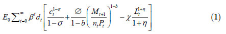
In this function variables n_t and d_t in utility function respectively are expectation shock that has shown as fluctuation in IS equation and another is money demand shock; that both of them follow statistic process (Novales et al, 2009).
Design of constraint budget of household
In household budget constraint design, first investment sector should divide to two parts. Investment part is on land and another part is on physical capital. On other hand, therefrom land as production factor should enter to production function, Households achieve revenue from giving rights of land and physical capital use, so its constraint will include land and physical capital. Therefrom taxing focus on revenue, so this system will operate on revenue in budget constraint.
For imposing unemployment, in the start that model has been formed, unemployment will enter to structure of model using defined parameters. Unemployment entry is formed according to parameter that is expressed during modeling. Actually, unemployment demonstrates itself as percent of variable that is deducted from its first quantity. For clearly explain of imposing unemployment if variable x_(t+1)be quantity of factor in t+1 period:

In this equation ñ quantity is parameter of imposing unemployment and ñx_t is unemployment quantity that is deducted from x_t variable in existence of this factor possibility. If numerical ñ parameter quantity equivalent to zero, demonstrates non-existence of unemployment in model and if it’s contrary zero, demonstrates existence of unemployment in model.
In present study, explains revenue quantity of each factor to impose tax. Therefrom rent revenue of these factors by firms belong to households, taxing show itself in budget constraint and imposes on revenue of this unemployment by households. For clarify issue Q_t K_t has been assumed physical capital revenue; so, therefrom a percent of that will be unemployment or non-used basically a percent of revenue of physical capital will belong to quantity of incomplete employment. For taxing from this a percent, we will have:
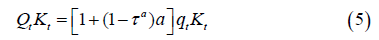
Above equation demonstrates physical capital total revenue subtract τ^a a proportion for each period that equivalent with gained percent of tax from revenue of quantity of imperfect employment in each period. This process can be repeated for physical capital on capital revenue with tax existence (that explained in household constraint sector), and taxing on land.
Household budget constraint is modeled according to economic growth (theory and numerical solution method) written by Novales et al. (2009). But, before budget constraint explanation, we should mention type of modeling of physical capital accumulation and also land accumulation as another production factor that derived from physical capital:
Investment equation in household budget constraint is in following form:

We have from physical capital accumulation:

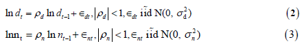
That a is quantity of non-used physical capital, δ is depreciation quantity and ν_t is investment shock that follow following process:

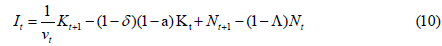
Now we write accumulation equation for land:

That Λ is unemployment quantity or non-used land. This equation demonstrates land quantity that involves in production (N_(t+1)) decrease with specified percent for profitability motivation that is the same motivation of imperfect employment in the end of each period. Mainly, N_(t+1) is expected stock of ready land for production that quantitative of that is incomplete employment according to incomplete employment in each period.
Concept of equation (9) can be clarified with an example. Active factory is assumed near empty land. This factory needs more space for expansion of production line to increase production capacity. So, it tries to rent or buy empty land. With assumption existence of inflation circumstances and incomplete employment in economy, since percent of growth of land price is more than growth of return of produced goods, so owner of land doesn’t rent or sell land to factory and saves it useless for motivation of more increase in prices. So, according to inflation and incomplete employment continuous trend, more lands will be out of production each year.
There is another point in equation (9) that land is modeled as its macroeconomic concept. This means that this factor modeled apart from its using concept such as agricultural, housing, industrial and other land and also depreciation isn’t considered for this factor despite of physical capital (Ostadzad & Behpour, 2015).
So, with replacement (7) and (9), equation (6) in budget constraint will be:
According to we assumed two situations in this study, so household budget constraint is modeled in two moods. In first mood budget constraint is modeled non-existence of unemployment or under-full employment assumption (although its parameter is in budget constraint but is assumed in zero calibration that is non-existence of unemployment mood) and in second mood under-full employment existence is assumed with imposing tax on it. So, first general concept of budget constraint is explained, then its different moods are modeled mathematically.
Households start itself with saving annual bond (B_t) and saving annual money (M_t) each t period. In the start of period households receive financial help or payment in T amount. After receiving this transfer, government’s bonds start to increase and these bonds convert to money for people. Households pay part of their money to buy government’s bonds B_(t+1) with annual price B_(t+1)/ ((1+i_t ) ) in next period, where i_t is annual interest rate. Remain money is paid for final good in price equivalent with P_t. At last households receive money D_t unit as receipt profit of factory of intermediate goods producer. Money equal to M_(t+1) and B_(t+1) generate in t+1 perid.
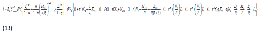
According to above definitions, household budget constraint in first situation is:

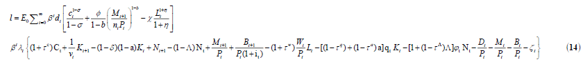
Also, budget constraint for second situation is:

According to budget constraint of two condition, unemployment quantity in production factors has been shown by a and Λ. Also, according to equation (5) definition tax quantity on revenue of this unemployment is formed in right side of budget constraint of second situation. Important point that is unemployment quantity exists in first situation but its quantity is considered zero in calibration sector.
Dynamic optimization for first situation
First, for solving optimization problem form of household, utility function should specify. In present study, household utility function is modeled based on advance macroeconomic written by Thomas Steger that includes consumption expenditure, real money balance and labor quantity. According to specifying form of household utility function, optimization problem is following lagrangian equation:
Important point in this sector is although quantity of non-used production factor in first situation is parametric, but their quantity considered zero in calibration sector. Due to this operational impact of unemployment existence without imposing tax on incomplete employment, it can be observed and analyzed by imposing some of unemployment in calibration.
Therefrom most changes were in base model in household sector and there is no change in firm and monetary and fiscal policy sector, so in next level we will solve optimization problem for household in second situation and then will optimize firms and monetary and fiscal sector between two situations in the same way.
Dynamic optimization for second situation
Firms
Firms: there is mass of homogenous firm that each of them hiring their labor for different goods production and sells its goods in exclusive competition market.
Final goods producer firms
Production function of final firm based on digitsit stiglitz index is assumed as following:
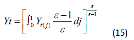
That Y_t(j) is production of jth intermediate firm. Requirements for intermediate firms to have competition power is ε<∞, because in this mood intermediate goods are incomplete substitute for each other. Purpose of final firm is choosing intermediate goods; as maximizes its profit (mainly, final good producer firm takes intermediate goods and sell them in competition market). Above problem presents as follows:
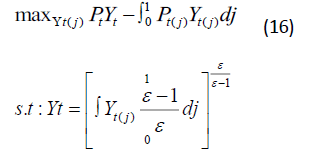
With replacement above constraint in objective function and converting that to irregular optimization, firstorder condition for optimization is:
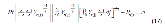
The point is quantity for P_t and P_t (J) is already assumed. The second phase in above equation is equal to Y_t^(1/θ). Therefore, optimal demand function is as follows:
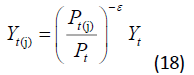
Equation (18) demonstrates that demand for each intermediate good depend on its relative price negatively and depend on total production positively. Also, condition ε>1 demonstrates exclusive competition firms' producer in elastic part of demand curve (Tavakolian & Sarem, 2016).
Intermediate goods producer firms
In this sector production is assumed function of physical capital, labor and especially land. Therefrom, unemployment is applied in physical capital and land sector in household sector; so, there is no need for re-application of unemployment in this sector.
In each period, jth intermediate goods producer firm hires L_(t(j)) unit of household’s sample labor equal to w_(t(j)) as wage, K_(t(j)) unit of physical capital equal to q_(t(j)) rent price and finally N_(t(j)) unit of land equal to φ_(t(j)) rent price to produce Y_(t(j)) unit of intermediate goods. This production function is in following technology form:
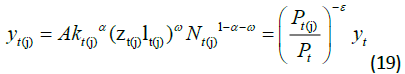
In above equation, ε is substitution elasticity between intermediate goods and Z_(t(j)) is technology shock that is common between entire intermediate producer firms and it follows below process:

Intermediate good substitutes to produces final goods incompletely. So, intermediate goods producer firms sell their goods to final goods producer firms in exclusive competition market that their price depend on final goods producer firms. Therefore, intermediate goods producer firms are face with price adjustment quadratic cost function (that in this study price Adjustment of Rotemberg (1982) has been used):
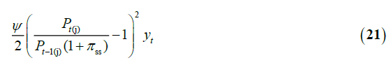
Where Ψ > 0 and πss is inflation in steady state (Novales et al., 2009).
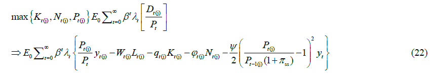
Finally, dynamic system form as lagrangian for jth firm:
Monetary policy
Monetary policy makes policy for annual interest rate of money based on Taylor rule that is based on NewClassic monetary model (Novales et al., 2009).

Fiscal policy
Fiscal policy is policy with tax on revenue of labor and capital and also consumption. If government faces budget deficit, publishes bonds, also pays transfers as Lump-Sum transfers. Therefore, budget constraint is modeled as follows (Novales et al., 2009):

Therefrom, there is taxing on unemployment in physical capital and land sector in this study, so taxes added to budget constraint.
Market clearing conditions
In this study, market clearing conditions is equal to General equilibrium of Keynes that production is equal to household’s demand for consumption and investment and also cost quantity for production:

Calibration of the parameters
Variable’s transform equations are extracted for Iran using variables quantity of Iran’s economy. Therefore, real data of economy of Iran should be used. Required data for present study is derived from different valid sources. Estimation quantity for parameter of present model is collected in follow table 1 according to real data of economy of this country.
| Parameters | Descriptions | Values | Sources |
|---|---|---|---|
| σ | Contrariwise intermediate consumption substitution elasticity | 1.5 | Motevaseli and coworkers |
| b | Contrariwise real money balance elasticity | 1.34 | Manzor and Taghipor |
| ε | Substitution elasticity between intermediary goods | 4.33 | Motevaseli and coworkers |
| φ | Fixed coefficient | 1 | Azam Ahmadian |
| α | Capital share from production | 0.55 | Ostadzad and Behpor |
| ω | Labor share from production | 0.01 | Ostadzad and Behpor |
| δ | Depreciation rate | 0.044 | Abolhasani and coworker |
| τq | Tax on capital | 0.052 | Rezaii and Molabahrami |
| τc | Tax on consumption | 0.049 | Rezaii and Molabahrami |
| β | Discount rate | 0.91 | Rezaii and Molabahrami |
| ψ | Price adjustment cost | 4.26 | Motevaseli and coworkers |
| ρz | Technology shock gap coefficient | 0.79 | Mehregan and coworkers |
| ρd | Preference shock gap coefficient | 0.66 | Manzor and Taghipor |
| ρn | Money demand shock gap coefficient | 0.554 | Manzor and Taghipor |
| ρx | Investment shock gap coefficient | 0.60 | Manzor and Taghipor |
| ρi | Interest rate importance coefficient in financial policy reaction function | 0.802 | Azam Ahmadian |
| ρy | Production importance coefficient in monetary reaction function | 0.4044 | Azam Ahmadian |
| ρπ | Inflation importance coefficient in monetary reaction function | 0.6941 | Azam Ahmadian |
| a | Imposed unemployment quantity in physical capital sector | %20 | Scenario making |
| Λ | Imposed unemployment quantity in land sector | %20 | Scenario making |
| τa | Imposed tax on unemployment in physical capital sector | %50 | Scenario making |
| τΛ | Imposed tax on unemployment in land sector | %50 | Scenario making |
Table 1. Calibrated parameters.
Due to non-existence of statistics study on quantity of non-used production factor such as physical capital and land, there isn’t any data for non-used land physical capital, so scenario making method used for these coefficients. Therefrom, in this study physical capital and land are close to each other from identity aspect, quantity of incomplete employment for both of them is 10% and for better influence of taxing on revenue of these, half of its quantity allocated for taxing that is equivalent with 5%.
Empirical results and IRFs analysis
In this section, first we categorize and compare results of three estimated moods of model. Three estimated moods include results of non-existence of non-used production factor, existence of non-used production factor and existence of incomplete employment in addition to tax their revenue.
Figure (1 to 5), respectively are concluded from five preferences, money demand, investment and technology shock and monetary policy that describe interest rate based on Taylor rule. These figures are dynamic path for non-existence of non-used production factor and existence of imperfect employment in addition to taxing on their revenue as two assumed situation. With comparing these path that indicate dynamic path of economy for basic variables, to attain steady state for each mood; it is observed absolute value of maximum and minimum point of transform curves had different fluctuations with increase of imperfect employment in production factor, for example due to influence of preference shock, absolute value of these points decreased but technology shock is caused increase in absolute value of points. Although, these fluctuations in each shock do not follow repetitive trend. But due to increase in rate of non-used production factor, range of these curves decrease. It shows due to increase in non-used production factor, speed of reaching to steady state increases. It can be said non-used production factor is caused faster withdraw of resources from economy cycle and decrease in its long path. More incomplete rate in these factors, shows it more (Manzoor & Taghipour, 2016).

Figure 1. IRFs of preference shock.

Figure 2. IRFs of monetary policy according to Taylor rule.

Figure 3.IRFs of investment shock.

Figure 4.IRFs of technology shock.

Figure 5.IRFs of money demand shock in action to liquidity.
Comparing table (2) with steady state quantity of production factor like capital (kss) and land (Nss) in three mentioned moods demonstrate quantity of imperfect employment decrease with increase in its rate in these factors in steady state that typically indicate unemployment in these factors. Due to this unemployment, real interest rate of this factors increase that is each unit of these factor’s value rate. So, demand surplus is generated for production factor with existence of unemployment and their supply will decrease. Sample of this decrease in supply can be observed in production quantity (yss) decrease in steady state.
On other hand, where taxing is imposed on under-full employment revenue, adjustment of quantity of unemployment in production factor can be seen. Due to this adjustment, value rate of each unit of production factor decrease and finally decrease in their supply will adjust. Sample of this adjustment can be seen in increase of production in steady state. Although, direct taxing from revenue of non-used production factor adjust unemployment in these factors, but their supply quantity won’t return to nonexistence of incomplete circumstances, so production level won’t return to non-existence of incomplete production factor circumstance.
In according to table (2) in compare with steady state of model, value rate of each unit of land (φss) equal with 0.11 in non-existence of unemployment that this rate increased to 0.31 with existence of imperfect employment and finally decreased to 0.27 with taxing again. This procedure can be seen in value rate of each unit of capital or in the same real interest rate (qss). This rate was equivalent with 0.15 in non-existence of unemployment that increased to 0.35 with imposing unemployment and adjusted to 0.31 after taxing.
| Title | Quantity | ||
|---|---|---|---|
| a=Λ | 20% | 20% | 0 |
| τa=ΤΛ | 50% | 0 | 0 |
| φss | 0.27 | 0.31 | 0.11 |
| qss | 0.32 | 0.35 | 0.15 |
| Nss | 6.41 | 5.41 | 38.96 |
| Kss | 7.11 | 5.66 | 37.39 |
| yss | 6.64 | 5.45 | 36.72 |
| iss | 2.95 | 2.41 | 1.65 |
| π ss | 2.60 | 2.11 | 1.40 |
| css | 3.71 | 3.04 | 35.07 |
| mss | 5.60 | 4.66 | 79.23 |
Table 2. Steady state quantity for non-existence of incomplete employment, existence of incomplete employment and existence of incomplete employment with tax on their revenue.
With this view that present model wants to analyze this unemployment in production factor that rent to firms by households, so it can be observed due to existence of unemployment value rate of each unit of produced factor increase and this increase in value rate or the same price, decrease exist production factor quantity among households, so decrease production and consumption and finally decrease utility and household welfare. The same analysis can be explained for real money balance quantity of households. So, with short view to table (2), it can be seen that real money balance quantity of households as one of utility factor among households is in positive form and decrease in existence of unemployment; so due to decrease in this factor, utility will decrease too and finally household welfare will decrease.
According to taxing quantity from unemployment in table (2) that its cause can be imperfect employment among households, it can be seen clearly that all economy basic variables except inflation and annual interest rate will justify. According to this point that taxing is regulator rules in economy sector, it can be seen that considerable decrease in value rates or price in production factor with considerable quantity of taxing from unemployment is equal to 50%. Therefore, it can be concluded if we assume household in situation without incomplete employment, the same situation that didn’t have speculative behavior institutionalized, they have more production, more real money balance and in result more consumption that these factors show more welfare of this type of situation.
According to mentioned points, another result can be concluded with comparing production level. Production level in non-existence of unemployment equivalent with 36.72 unit that decrease to 5.45 with existence of unemployment that is considerable quantity. Now, with imposing tax on unemployment production again increase to 6.64 level but don’t reach to non-existence of unemployment level. This is production gap or tax cost of government to avoid speculative behavior.
Therefrom government should establish organization for taxing or hires more labor fiscal organization to explores revenue quantity of non-used production factor and taxing from them, so part of labor and capital withdraw from production sector for this organization and use in taxing organization. Due to this cause, production level won’t return to non-existence of unemployment level even with 50% taxing.
With comparing mentioned quantities, negative impact of non-used production factor on consumption and production is specified. So, land and physical capital become stagnant in non-used production factor and don’t convert to production, revenue and finally consumption. In other words, this indicates the withdrawal of land and physical capital from the production cycle, but it doesn’t indicate the disappearance or conversion of these two factors into consumption. On other hand, non-existence of in-appropriate efficiency of taxing from revenue of incomplete employment indicate if no speculative action happens, there is no need to tax cost and economy of that situation will have more level of production, consumption and welfare.
Theoretically, the most important aspect of this study is existence of production function with land factor in NewKeynesian model. This factor hasn’t considered in majority of other studies, while it has emerged with physical capital in terms of nature, but has been included important share of production. Combination of incomplete employment demonstrates influence of both non-used land and physical capital and therefrom both of them exist in Iran’s economy, this model is simulated good approximation to evidence of Iran’s economy. It is considered that these models indicate negative impact of imperfect production factor with decrease in production level that resulted from land and physical capital unemployment. Direct result of existence of imperfect employment in these factors shows increase in price of both factors in lower production level with non-existence of it in economy. This result two conclusion that finally will conclude labor unemployment. First, increase in share of production, decrease labor price because of demand surplus in physical capital and second, lower production level needs fewer labor. In aggregation these two flows result unemployment in labor. In the case of production factor unemployment, although share of production factor increases in production in these circumstances but lower land and physical capital is used in proportion to non-existence of incomplete employment, land and physical capital because of decrease in production level. Also, production factor become unemployment.
Also, in case of taxing it can be said that although this policy, is policy of most of economy systems as regulator rules but their impact isn’t much to return economy circumstance to non-existence of incomplete employment circumstances with existence of adjustment in production factor price and maybe indirect taxes can have influence on it. So, it can be said if we justify speculative actions, there is no need to bear more cost to economy. So, communities that does not have any speculative actions, is entered all their resources to production cycle and economy and finally experience more level of consumption, utility and welfare.
Abolhasani A, Ebrahimi I, Pour Kazemi MH, Bahrami Nia EB (2016). The effect of oil shocks and monetary shocks on production and inflation in the housing sector of the Iranian economy: New Keynesian dynamic stochastic general equilibrium approach. Quarterly Journal of Economic Growth and Development Research. 7: 113-32.
Ahmadyan A (2016). Modeling a dynamic stochastic general equilibrium model for the Iranian bank withdrawal. The journal of economic policy. 7: 77-103.
Bakhshi Dastjerdi R, Rahimi R (2017). Studying the Effects of Hording on Production and Welfare Designing a Dynamic Stochastic General Equilibrium Model for Iran’s Economy. Journal of Economic Research (Tahghighat-E-Eghtesadi). 52: 789-820.
Bastani Far I, Mirzaei R (2014). Analyzing the roots of the stagflation in the Iranian economy and providing solutions. Journal of Monetary and Banking Research. 21: 361-80.
Central Bank of IRI (2017). Economic time series database.
Du J, Peiser RB (2014). Land supply, pricing and local governments' land hoarding in China. Regional Science and Urban Economics. 48: 180-9.
Indexed at, Google Scholar, Cross Ref
Feiger G (1976). What is speculation?. The Quarterly Journal of Economics. 677-87.
Indexed at, Google Scholar, Cross Ref
Karau S (2020). Buried in the vaults of central banks: Monetary gold hoarding and the slide into the Great Depression. Available at SSRN 3767290.
Indexed at, Google Scholar, Cross Ref
Kociecki A, Kolasa M (2018). Global identification of linearized DSGE models. Quantitative Economics. 9: 1243-63.
Indexed at, Google Scholar, Cross Ref
Manzoor D, Taghipour A (2016). A dynamic stochastic general equilibrium model for an oil exporting and small open economy: the case of Iran. Journal of Economic Research and Policies. 23: 7-44.
Mehregan N, Isazadeh S, Abbasian E, Faraji E (2016). Estimating of the Equilibrium Situation of Iran’s Economy within RBC Models. Quarterly Journal of Applied Theories of Economics. 3: 1-22.
Motavaseli M, Ebrahimi I, Shahmoradi A, Komijani A (2011). A new Keynesian dynamic stochastic general equilibrium (DSGE) model for an oil exporting country. The Economic Research. 10: 87-116.
Nakhli SR, Rafat M, Bakhshi Dastjerdi R, Rafei M (2020). A DSGE Analysis of the Effects of Economic Sanctions: Evidence from the Central Bank of Iran. Iranian Journal of Economic Studies. 9: 35-70.
Indexed at, Google Scholar, Cross Ref
Novales A, Fernandez E, Ruíz J (2009). Economic growth: theory and numerical solution methods. Berlin: Springer.
Ostadzad AH, Behpour S (2015). A new approach to calculate the time series of capital stock for Iranian economy: The recursive algorithm method using genetic algorithms (1959-2011). Journal of Economic Modeling Research. 5: 141-78.
Rezaii I & Molabahrami A (2017). Impact of Fiscal Policy on Dynamic of Growth, Capital and Consumption Based on an Optimal Growth Model: in Case of Iran and Countries of East Asia. Quarterly journal of Economic Research (Stable Growth and Development). 1: 73-94.
Rotemberg JJ (1982). Sticky prices in the United States. Journal of political economy. 90: 1187-211.
Indexed at, Google Scholar, Cross Ref
Schumpeter JA (2006). History of economic analysis. Routledge.
Indexed at, Google Scholar, Cross Ref
Seyed NS (2014). An examination of housing bubble and speculation in urban areas of Iran.
Statistical center of Iran (2017). Household, expenditure and income.
Stiglitz JE, Rosengard JK (2015). Economics of the public sector: Fourth international student edition. WW Norton & Company.
Tavakolian H, Sarem M (2016). DSGE models in DYNARE (modeling, Solution and Estimation for Iran).
Toutounchian I (2011). Islamic money and banking: Integrating money in capital theory. John Wiley & Sons.
Indexed at, Google Scholar, Cross Ref
Walsh CE (2017). Monetary theory and policy. MIT press.
Yang X, Wu Y, Shen Q, & Dang H (2017). Measuring the degree of speculation in the residential housing market: A spatial econometric model and its application in China. Habitat International. 67: 96-104.
Indexed at, Google Scholar, Cross Ref
Zheng M, Wang H, Wang C, Wang S (2017). Speculative behavior in a housing market: Boom and bust. Economic Modelling. 61: 50-64.
Indexed at, Google Scholar, Cross Ref
Citation: Ashkan I & Homayun R (2022). Planning a DSGE model for economy under state of under-full work underway variables: Another keynesian methodology. JRIBM. 9: 017.
Copyright: © 2022 International Research Journals This is an open access article distributed under the terms of the Creative Commons Attribution License, which permits unrestricted use, distribution, and reproduction in any medium, provided the original work is properly cited.